A pair of new related sequences of integers

Projects

A) 1, 1, 1, 1, 1, 1, 1, 1, 1, 1, 1, 1, 2, 2, 1, 2, 1, 4, 1, 1, 1, 1, 2, 1, 1, 1, 1, 1, 1, 1, 1, 1, 1, 1, 1, 2, 1, 4, 1, 1, 1, 2, 2, 1, 1, 1, 5, 1, 1, 1, 1, 1, 3, 3, 1, 3, 1, 1, 1, 7, 3, 1, 1, 1, 2, 1, 2, 1, 1, 1, 2, 1, 1, 1, 1, 3, 1, 1, 2, 2, 1, 3, 2, 2, 1, 4, 1, 1, 2, 2, 1, 1, 2, 1, 1, 2, 1, 3, 2, 2…
and
B) 1, 1, 1, 1, 1, 1, 1, 2, 5, 3, 1, 1, 1, 1, 2, 1, 2, 1, 3, 1, 1, 1, 1, 3, 1, 3, 3, 3, 4, 1, 2, 1, 2, 3, 1, 2, 1, 1, 1, 2, 1, 1, 1, 3, 1, 1, 1, 3, 3, 2, 3, 3, 1, 1, 5, 4, 3, 2, 3, 1, 7, 3, 3, 1, 1, 2, 1, 1, 1, 2, 2, 1, 2, 1, 2, 3, 1, 2, 3, 4, 1, 1, 1, 1, 2, 1, 5, 3, 1, 1, 3, 2, 3, 1, 3, 3, 4, 1, 4, 1…

What are these sequences, and what links them? Well, if you take the prime numbers in order, and sort each of their digits and then count how many factors each of these numbers has you’ll find either sequence A or sequence B depending on if you sorted the digits highest first or lowest first. The 1s represent numbers which are primes. The first few prime numbers only have 1 digit, so sorting the digits gives the same number, then there is 11, which sorted is still 11, and 13 which can be sorted to 13 or 31, both of which are prime. 19 is the first prime number, which when sorted highest to lowest gives a composite number.

A property of this pair of sequences is that, at least up to 9592 digits, the sum of the first n digits of B is greater than A. This is expected as the intermediate values, the sorted prime digits, of B are 1 larger and 2 more likely to have 0s or 2s at the end of them (since 0 and 2 are both small numbers and guarantee numbers to be composite). Larger numbers are more likely to have more factor since there are more available combinations. I don’t know this result to be true for all N, it is a conjecture.

I’m hoping that the sequences get accepted to the Online Encyclopedia of Integer Sequences (OEIS) which is the goto place for sequences like this to be sorted so that people can cross reference. If they do get accepted then they’ll be sequence A326952 and A326953, respectively. However, the OEIS curates the sequences that they list carefully so as not to include arbitrary sequence which no-one else will find interesting. I don’t know if other people will find this interesting.

Excitingly, as of the 25th of August, they have both been approved https://oeis.org/A326952 and https://oeis.org/A326953

Plot of the cumulative sum of each of the sequences
Plot of sequence A against sequence B for the first 4796 terms

Computer Controlled Macro focusing rail

Macro Photography, Photography, Projects
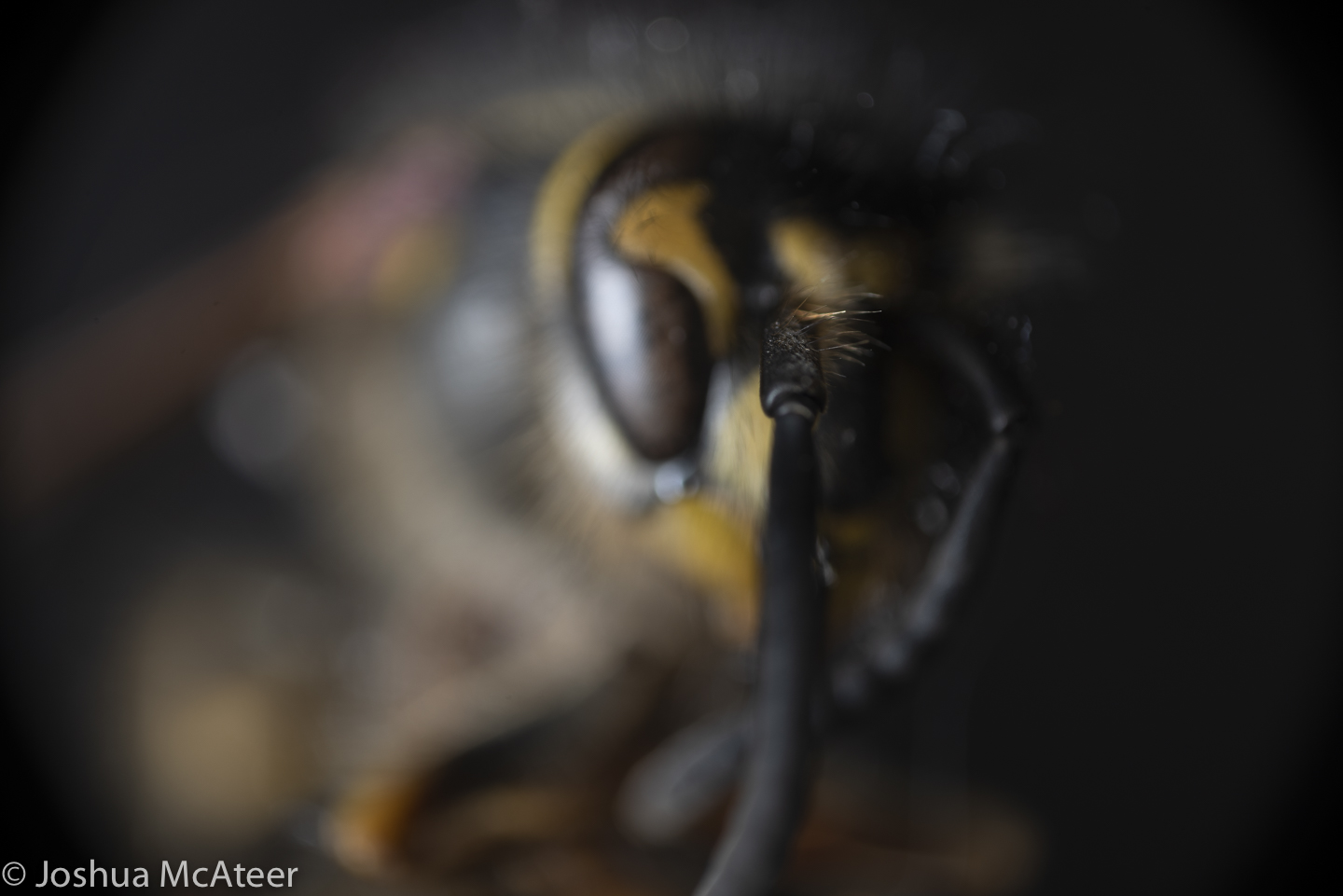
Stack of 128 frames of a wasp using a 3.7x 0.11NA objective on a Pentax K-1

Focus is often used creatively in photography to separate the subject from the background of an image. In microscopy ‘optical sectioning’ to resolve details out of the plane of the image. In macrophotography, however, we often want to capture images which are pin-sharp front to back. Doing this is quite hard.

The depth of focus is very narrow at high magnification. In fact, in the wasp portrait the depth of focus was only 58 microns, or only 0.058mm. You can see what a single image looks like bellow. Only few hairs are in focus. In total for this photo I took 128 images in 20 micron steps.

Single frame from stack

It’s pretty hard to move in 20 micron steps by hand, so for a little while I’ve been putting together a focusing system.

Version 1 was just a z-axis rail for a CNC machine. A rail with a carriage supported on it, with a screw thread and a like-threaded insert on the carriage, and a stepper motor. This was controlled by an arduino and stepper driver. The camera was set up with an interval timer, and the arduino code had periods in it for the camera to take a photo.

This setup had several disadvantages, securing the camera to the camera was difficult. an M5 to 1/4″ bolt was used, but this didn’t allow for the camera to be securely fastened. Also, the minimum step size was ~50µm which wasn’t fine enough. Lastly, the camera needed to stay in sync with the arduino, which was achieved by starting the arduino code a few seconds before the camera, not ideal.

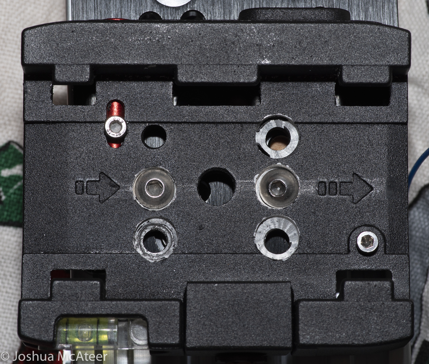
Version 2 has a number of improvements. By cannibalising a shutter release cable I’ve been able to control the camera from the arduino, by just bringing a pin high. I also drilled out a tripod base plate to give sufficient clearance for the camera plate to slide into it, while everything is bolted together. Lastely, I swapped out the threaded rod for a M8 fine pitch rod. This rod has a pitch of 1mm, and only 1 thread cut into it, instead of the ~2.5mm pitch and 4 threads cut into the rod I was previously using. This improves the stepping precision by a factor of 10. A single step on the new system is only 5µm, which is only about 10 wavelength of light.

The thread was cut into a small block of wood which was pre-drilled with an 8mm hole. The wood offers quite a lot of resistance, but also doesn’t produce any backlash.

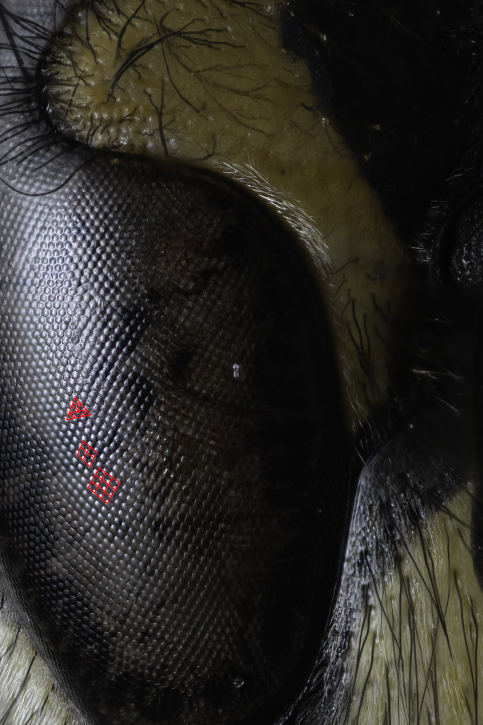
1:1 zoom of the eye of the wasp. 1px is 1µm in size. The facets of the compound eye are most interesting as they transition from the hexagonal packing into a square packing.

Mounting unusual lenses on digital cameras

Macro Photography, Photography, Photography Equipment, Projects
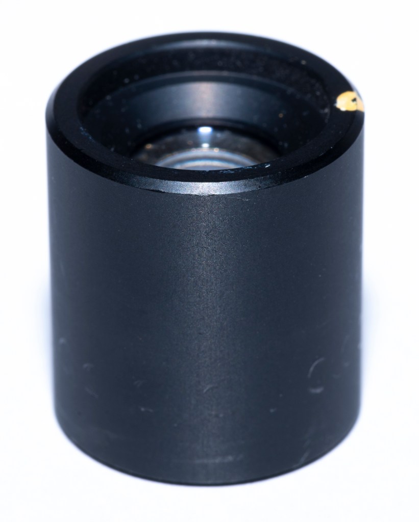
lens recovered from Polaroid Sprintscan 35

Pleasing effects can often be found when using unusual lenses on modern digital cameras. Sometimes they give a highly aberrated image which is useful in creative situations, sometimes the history of the lens enhances the image in a meaningful way, and sometimes the unusual lens offers a quality which is not possible with typical lenses from first party manufactures.

The last instance is often the case with macrophotography. Many people use objectives to photograph small insects as they offer much higher magnification ratios and resolution than macro lenses. Occasionally, lenses used for obscure purposes in industry can find use in various areas of photography. Surplus aerial photography lenses, such as the Kodak Aero-Ektar are highly sought after for their high resolution and high speeds over large flat film planes. Occasional lenses with have excellent performance are found for macrophotography.

It is one of these which I have acquired recently from an old film scanner. Film scanners image a flat sheet of film onto a flat sensor at high resolution. Unlike lenses for general photography they are optimised for magnification ratios of around 1. Most photography lenses are optimised for a magnification of almost zero.

lens recovered from Polaroid Sprintscan 35

Mounting a lens can be easy. Adapters often exist allowing a camera lens to be mounted on other cameras. However, when we look at older lenses, or lenses which were designed for industrial use the adaptation is more difficult.

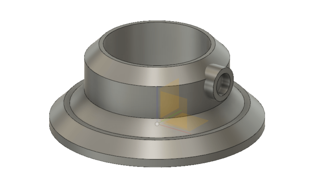
CAD model of the lens holder

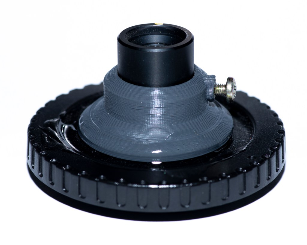
In order to mount the lens securely, I designed a small device to securely hold the lens. The bore has 0.5mm of clearance for the lens barrel, and a flange at the base so that the lens can be reliably positioned the same distance from the sensor. This was 3D printed by a friend of mine. There is also a place for a grub screw to be installed so as to secure the lens in place. The base is so sized so that it may be bonded to a body cap. The injection moulding used on the body cap left the inside surface shiny, this was sanded to reduce reflections. The body cap can the be fitted to a set of bellows or extension tubes.

3D printed lens hold affixed to body cap and with a screw to hold the lens in place
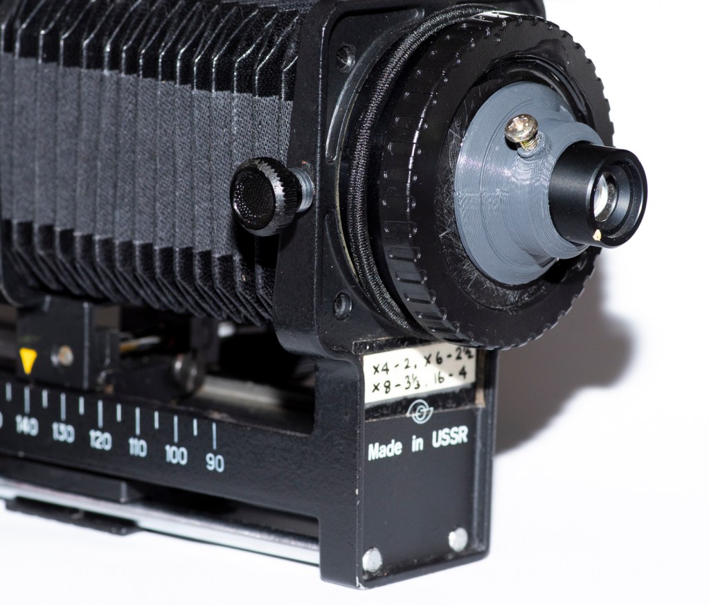
Lens mounted to an old set of bellows. These bellows are backwards, so that the remaining rails are on the camera end.

I was surprised to realise that the top of the body cap was quite convex. This cased two problems. Firstly, the contact area which the lens holder made was rather small, and secondly, it would slide about as the glue dried. To compensate for the first issue I used quite a lot of adhesive. To compensate for the first I used a quick curing epoxy resin. This turned out not to be so quick curing, and I spent about 30 minutes poking the parts into alignment.

I intend to test the lens both ways around and at different magnifications. I don’t know exactly what magnification it will perform best at, presumably at it’s design magnification. However, it may surprise us. The lens is not a symmetric design, the front (dot end) has a convex element, the rear surface is plano.

I took the lens out for a short while and tried to photograph some insects. Unfortunately, I didn’t bring my flash light guide, so most of the picture turned out greatly under-exposed. The lens is not exceedingly sharp, at least, not at the magnifications which I tested it at. However, this is not a well designed resolution test (that will come later).

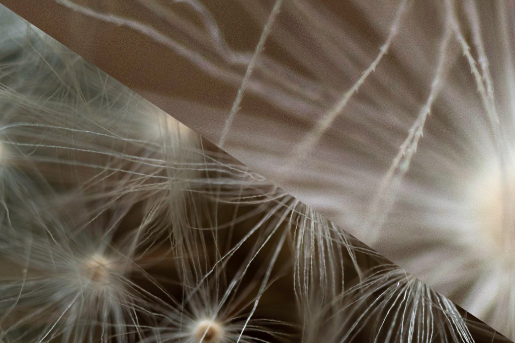
Full image (resized) and 100% zoom on a 36MP full frame sensor

As can be seen from the above frame, the lens is not sharp to the pixel. However, it shows nice contrast and has very little longitudinal chromatic aberration.

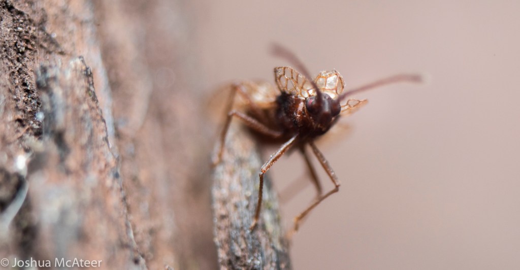
Not many insects would stay still for me. This guy did, but he was really small.

The insect above was very small. I’d be interested to know what species it is. Part of the issue with this photo is the due to a heavy exposure pull due to a lack of flash power. The Pentax K-1 isn’t known for its dynamic range, but this is pulled 3.5 stops, and I don’t think it is so bad. I tried a few different magnifications, but I didn’t keep track of it. The working distance is quite short, but this is also a lot higher magnification than my macro lens.

The resolution is probably what I should expect. The scanner that this lens came from was a 2,700 dpi scanner and the resolution of my sensor is 5,200 dpi, so it isn’t surprising that the sensor out resolves the lens. However, image space resolution isn’t the only important property.

JPEG artifact removal with Convolutional Neural Network (AI)

Uncategorized

JPEG images, at high compression ratios, often have blocky artefacts which look particularly unpleasant. JPEG images look particularly bad around the sharp edges of objects.

There are already ways to reduce the artefacts, however, these methods often don’t use very sophisticated techniques, only using the information from adjacent pixels to smooth out the actual transition between the blocks. An example of this can be found in Kitbi and Dawood’s work https://ieeexplore.ieee.org/document/4743789/ which gave me the original inspiration for this.

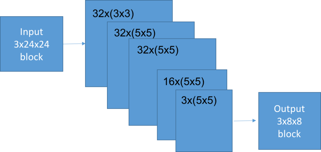
An alternative way is to use a convolutional neural network (CNN) to intelligently estimate an optimal block given the original block and the eight surrounding blocks. And then tile over the image to estimate the optimal mapping for each block.

The network design was a 5 layer fully convolutional one, using only small filters. Several different architectures were used, which all gave largely similar results. The compromise between effectiveness and speed (i.e. 1/size) was found with a small network with only 57,987 parameters. Training the network was surprisingly fast, taking only a few hours without a GPU.

The network takes in full colour information and outputs the full colour too. The reason for this is to use all of the possible information. The colour channels are highly correlated with one another. It would be possible to train the network on monochrome images, but that would lose the relation which naturally exists.

So, does it work?

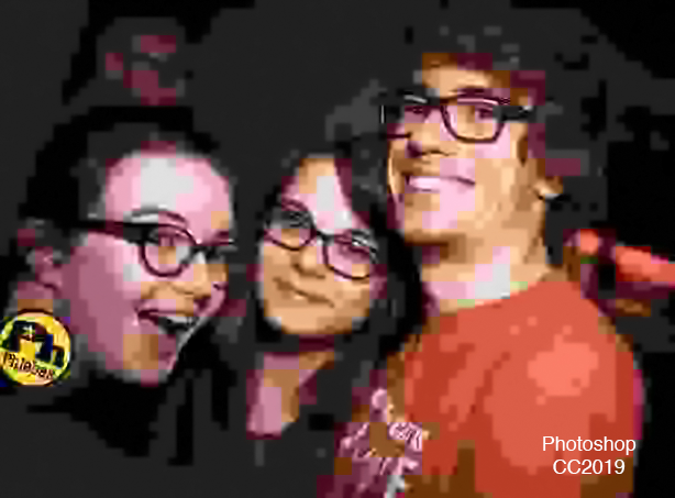
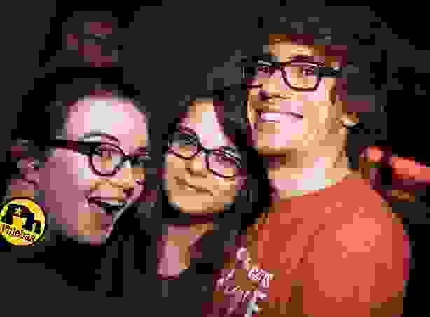
In my opinion, yes it does work. I think my method performs best when there are complicated edges, such as around glasses, or on hairs which are resolved as partial blocks. It works least well, in comparison to the method which photoshop currently uses, when there are large smooth areas.

Text was not present in the training data set. So the poor effectiveness of the network on text is not a significant point of comparison. The above images are quite small. A larger example is below, along with a zoomed in video comparing the original, JPEG, photoshop artefact removal, and my method.

I did calculate root mean squared error values one point comparing the network performance with the JPEG image to the original. In some cases the network was reliably out performing the JPEG – which is impressive, but not too surprising, as this was how it was trained. I don’t think that those sorts of values are too important in this case. The aim isn’t to restore the original image, but to instead reduce the visual annoyance of the artefacts.

If you really wanted to reduce the annoyance of the artefacts you should use JPEG2000 or else have a read of this paper https://arxiv.org/pdf/1611.01704.pdf

Photographs from Birdworld

Photography

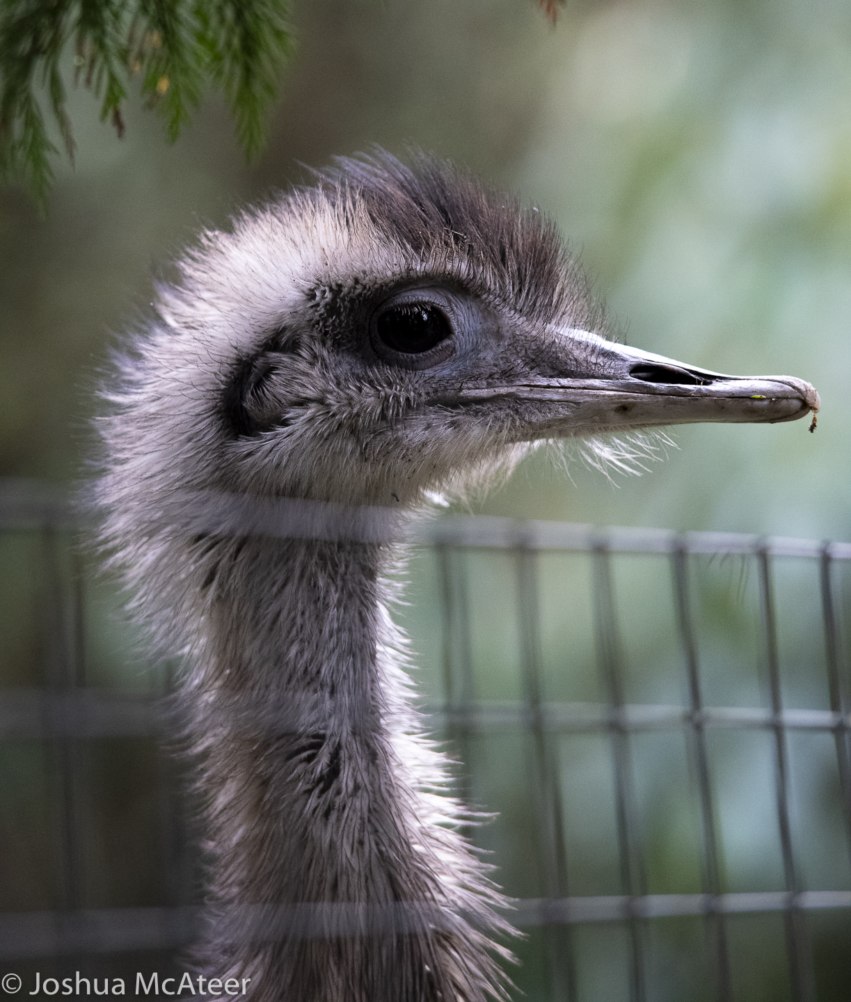
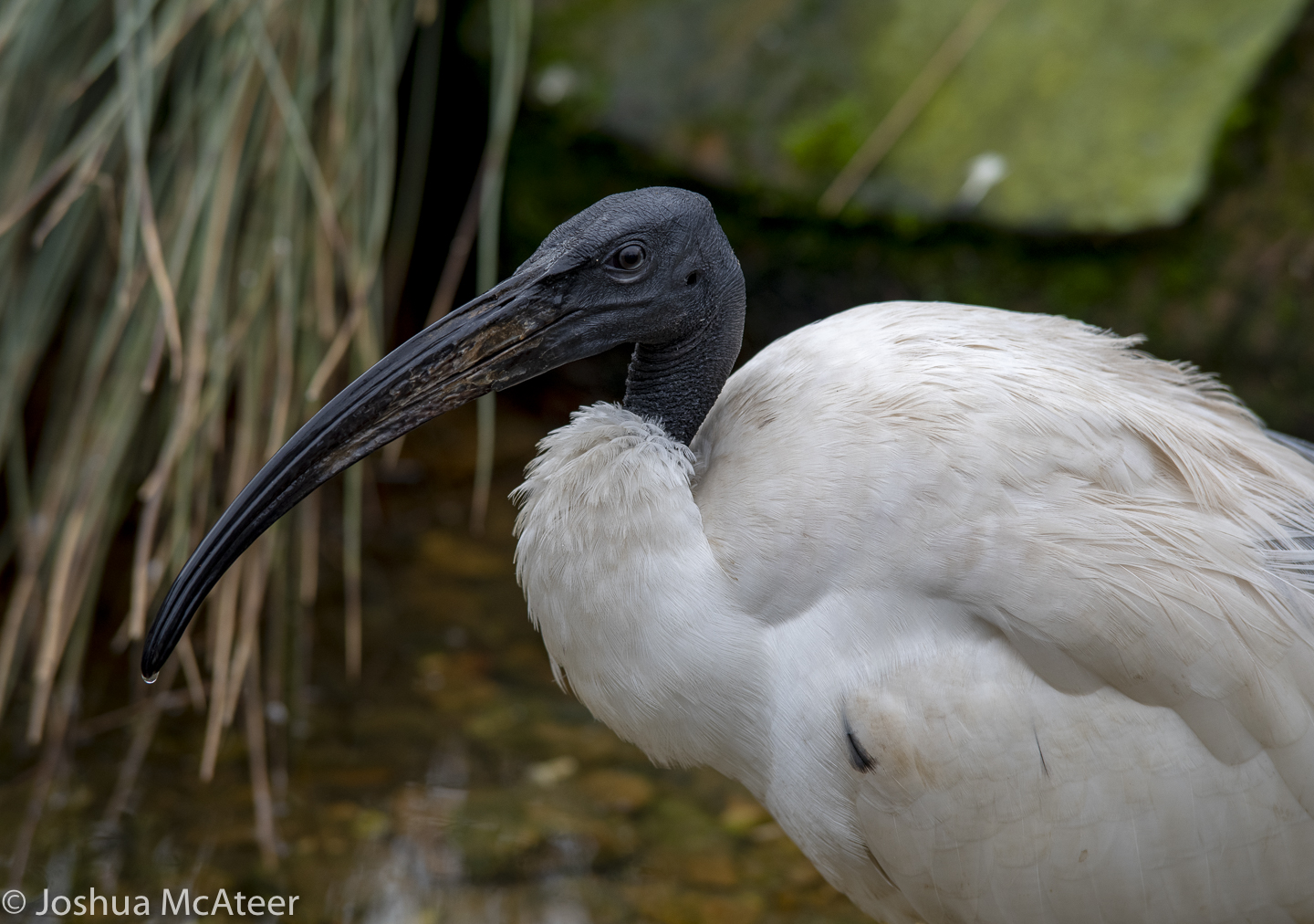
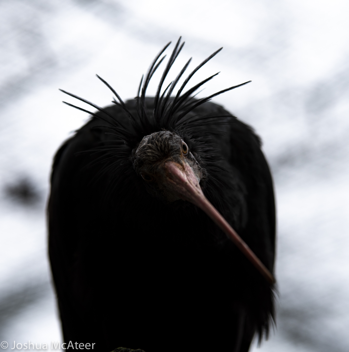
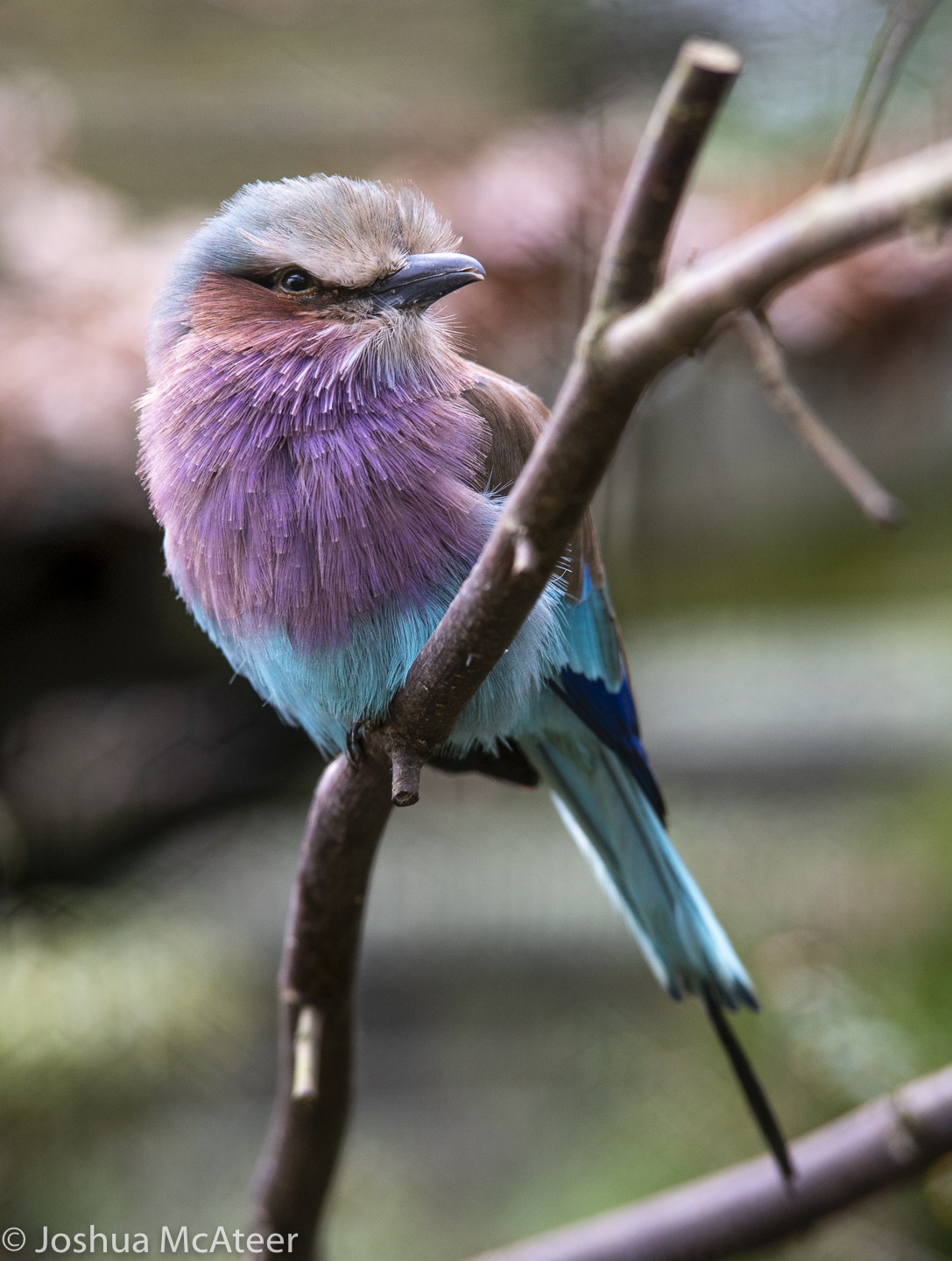
Over Christmas two photography related events happened. I acquired a 70-200, and I also went to Birdworld. These are some of the results. I really liked the lens (an older tamron) it’s quick to focus and brilliantly sharp at f4. The screw af is quite loud though and swapping between manual and autofocus is slow on pentax cameras.

My keep rate was about 7% for this outing, which is pretty good for me. Hopefully, as I become better acquainted with the lens that’ll go up.

The focus on the lens is a little slower than my SDM lens. But it is still snappy. I found that, to nail focus on the exact part of the eye I wanted, I needed to manual focus when the scene had foreground elements such as mesh or fence – which is completely normal.

Linify: photographs to CNC etch-a-sketch paths

Projects

Linify: def. to turn something into a line.

I saw someone the other day using a variable density Hilbert curve to transform an image so as to be projectable using a laser and galvo mirror setup, this was on the facebook page Aesthetic Function Graphposting.

That kinda stayed in the back of my mind until I saw This Old Tony’s youtube video about making a (computer numeric controlled) CNC etch-a-sketch. The hardware looked great, but he was just using lame line sketches of outlines, the kind of limited images which you’d expect from an etch-a-sketch.

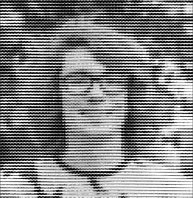
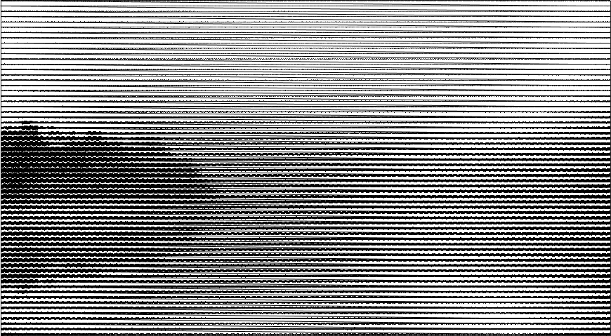
So, I put together a lazy easy way of turning a photo into a single line. Here is an example of my face. If you move quite far back from the image, it looks pretty good.

It uses a variable amplitude sinewave patches, which have a whole number of periods. Sine waves are used due to their simplicity and their periodicity. The same effect could be achieved with other periodic waves, in fact, square waves may be more efficient for CNC applications, as fewer commands would need to be issued to the orthogonal control axes.

The image is first downsampled to a resolution around 64 px on an edge. Then, for each pixel in the downsampled image, an approximate sinewave is found. Blocks of sine waves are added to a chain, which runs over the whole image. Currently, it raster scans, but it would be pretty easy to go R->L on even and L->R on odd. To improve the contrast, the downscaled image is contrast stretched to the 0-1 interval, and then each intensity value is raised to the (default) power of 1.5, this gives a little more contrast in the lighter regions and compensates somewhat for the low background level and the non-linear darkening with greater amplitude. This could be tuned better. 

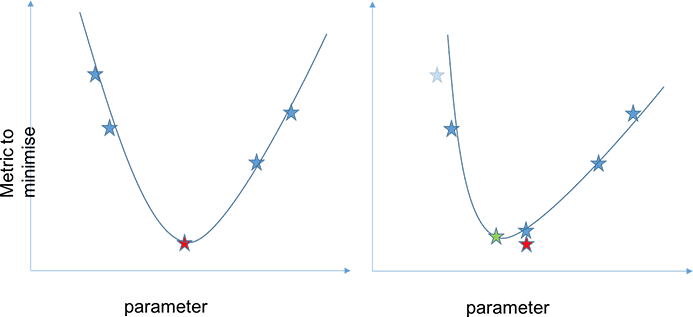
There are several factors which alter the contrast. The cell size, frequency, number of rendered points, linewidth, and also the gamma-like factor applied to the image before the linify. Images were then optimised by adjusting the gamma-like factor. Optimal values were found between ~0.75 and ~1.65. Higher values were better for darker images. Successive parabolic interpolation (SPI) was used, four values were selected at random, and their error with respect to the original image was found. These values were then used to fit a parabola, and the minima of the parabola were used as a new point. This process was iterated with the four best values being used for the fit. This process can be seen in the figures below. In the first figure, four points (the blue stars) are found. The first parabola is fitted, and the red point is the predicted best parameter value. In the second figure, the blue star shows the true value of the metric we are trying to minimise, it is slightly different than predicted. A new estimated best parameter value (green) is found. And so on. To ensure that the parabola is only used near the minima of the function, the points farthest from the minima are discarded. Typically, only three points are used, my implementation uses four for robustness, which is helpful as the curve is non-analytic and non-smooth.

A few starting locations were checked to ensure that the minimum found was global. This kind of root finding, SPI, is very simple and commonly used. It converges faster than a basic line search (about 33% faster) but does not always converge to the local extremum. Parabola are used, as the region around any minima or maxima of any function can be approximated by a parabola, which can be observed by the Taylor expansion about an extremum.

Whilst we have a non-linear intensity response and some artefacts from the process, it is much easier to get this kind of process to well represent real images than the skittliser process, as we have a wide range of possible intensity levels.

Of course, one of the issues with using this method on something like an etch-a-sketch is the extremely long paths taken without any kind of reference positions. Modifications could be made internally to an etch-a-sketch to have homing buttons which would click at certain x or y positions, thus giving the control system a method of resetting itself at least after every line. A much more difficult, but potentially interesting closed-loop control system would be using information from a video feed pointed at the etch-a-sketch. Taking the difference of successive frames would likely be a good indication of the tip location.   

Finally, here is a landscape photograph of a body of water at sunrise. Just imagine it in dusky pink. 

Photographs from NNT Heather

Photography

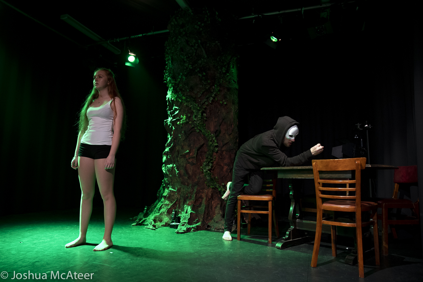
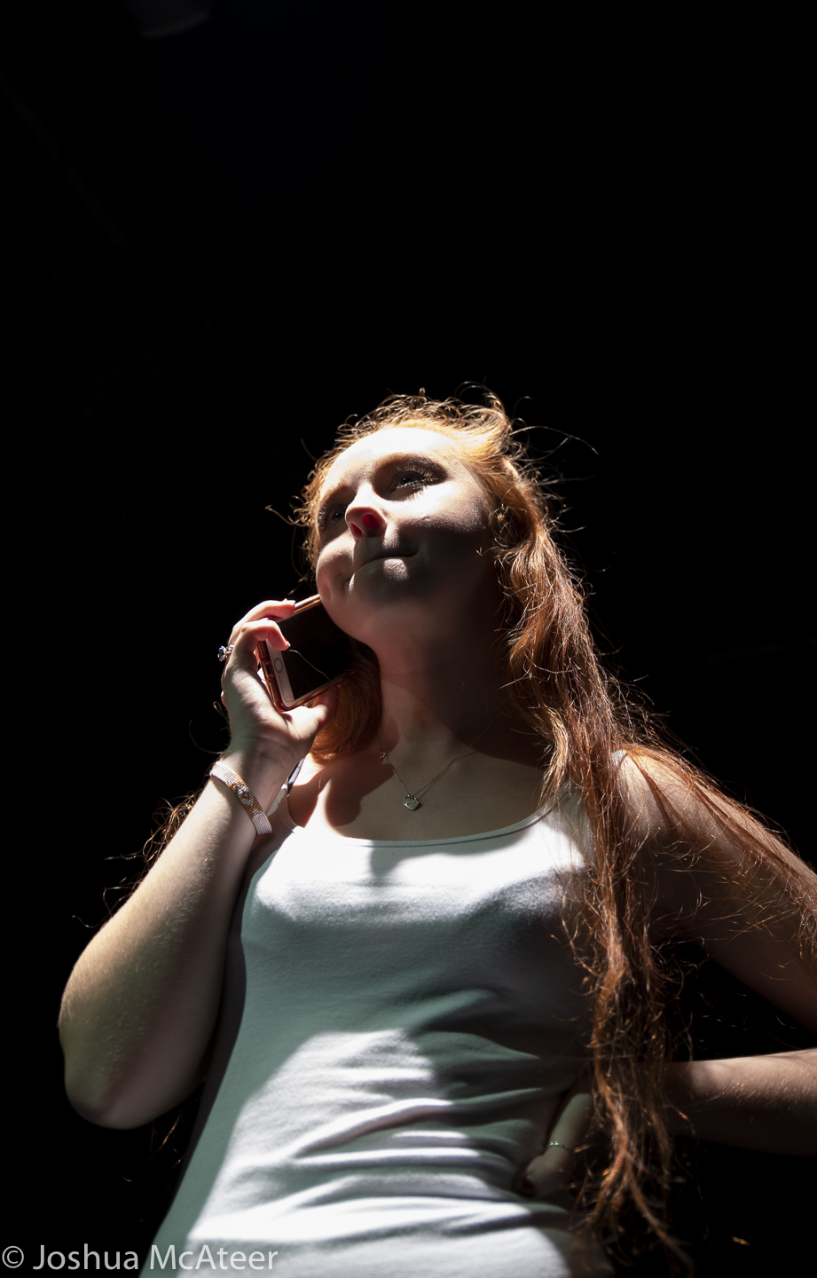
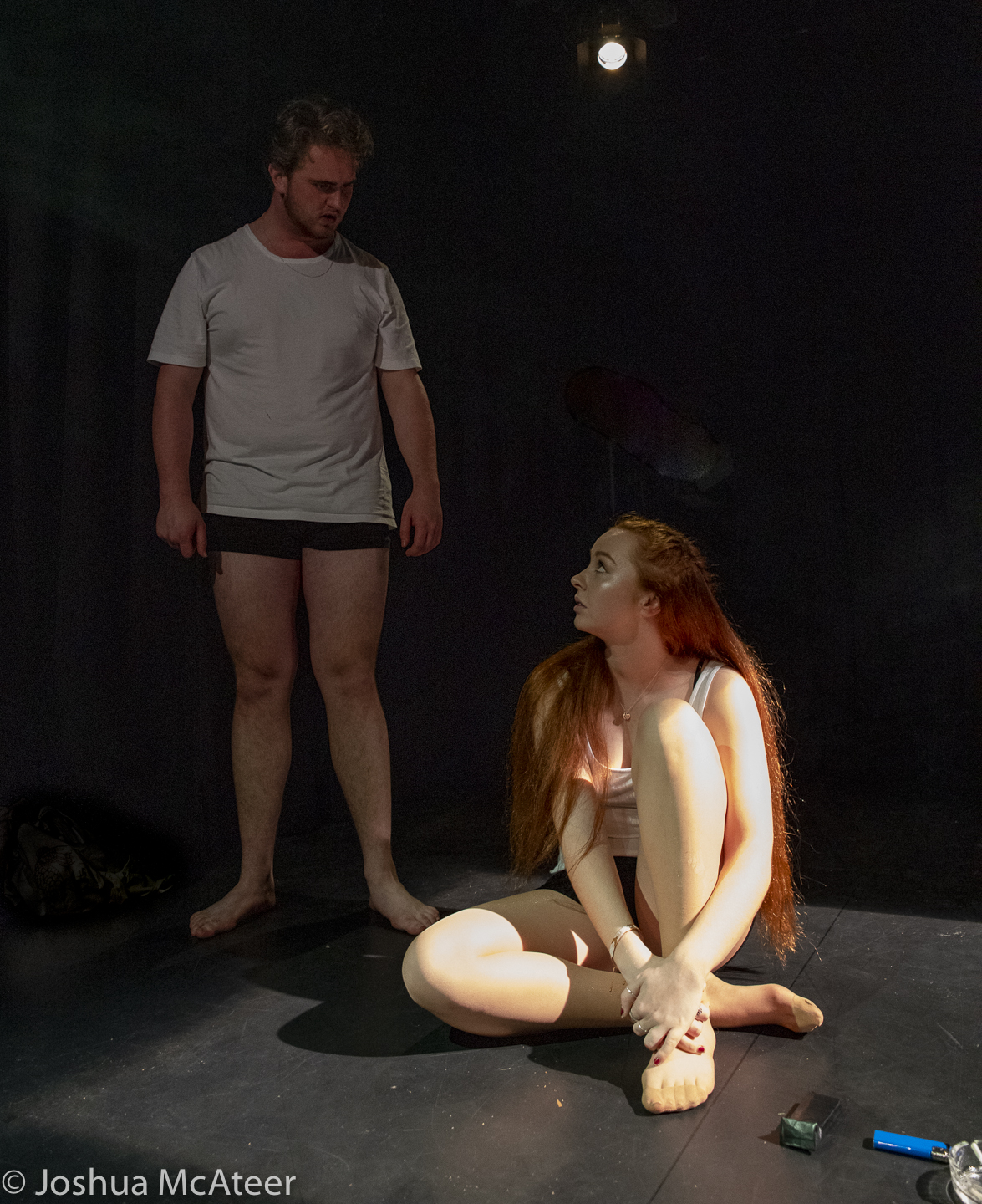
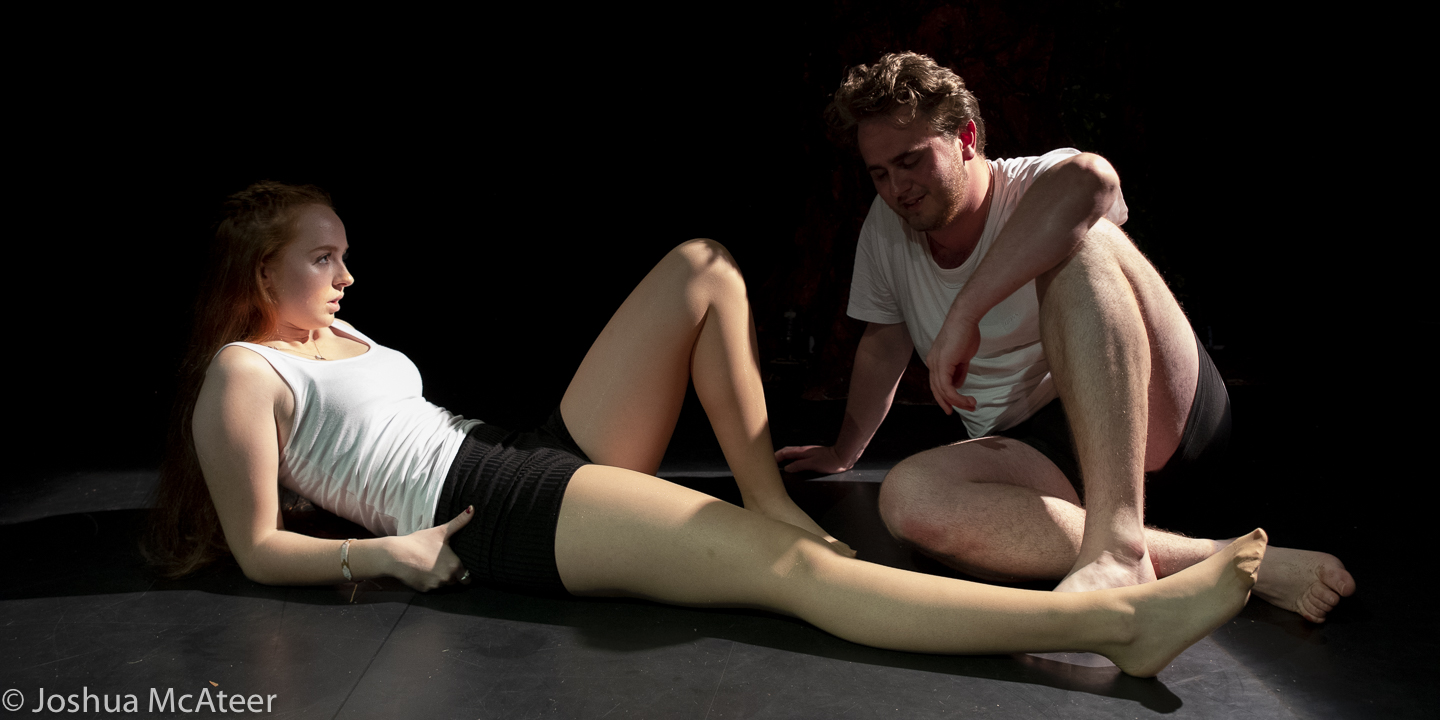
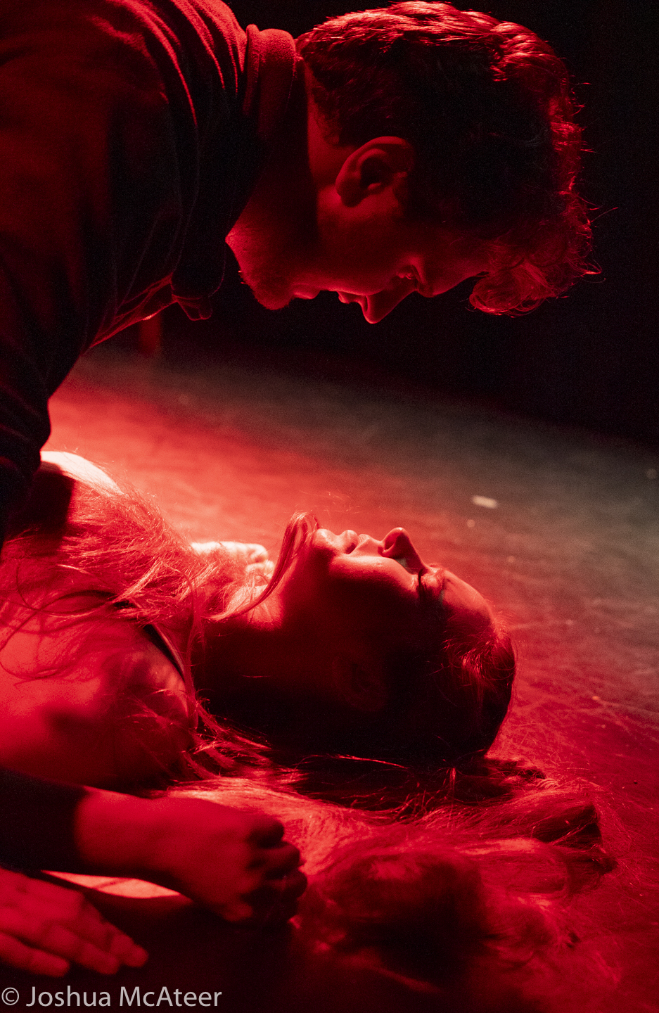
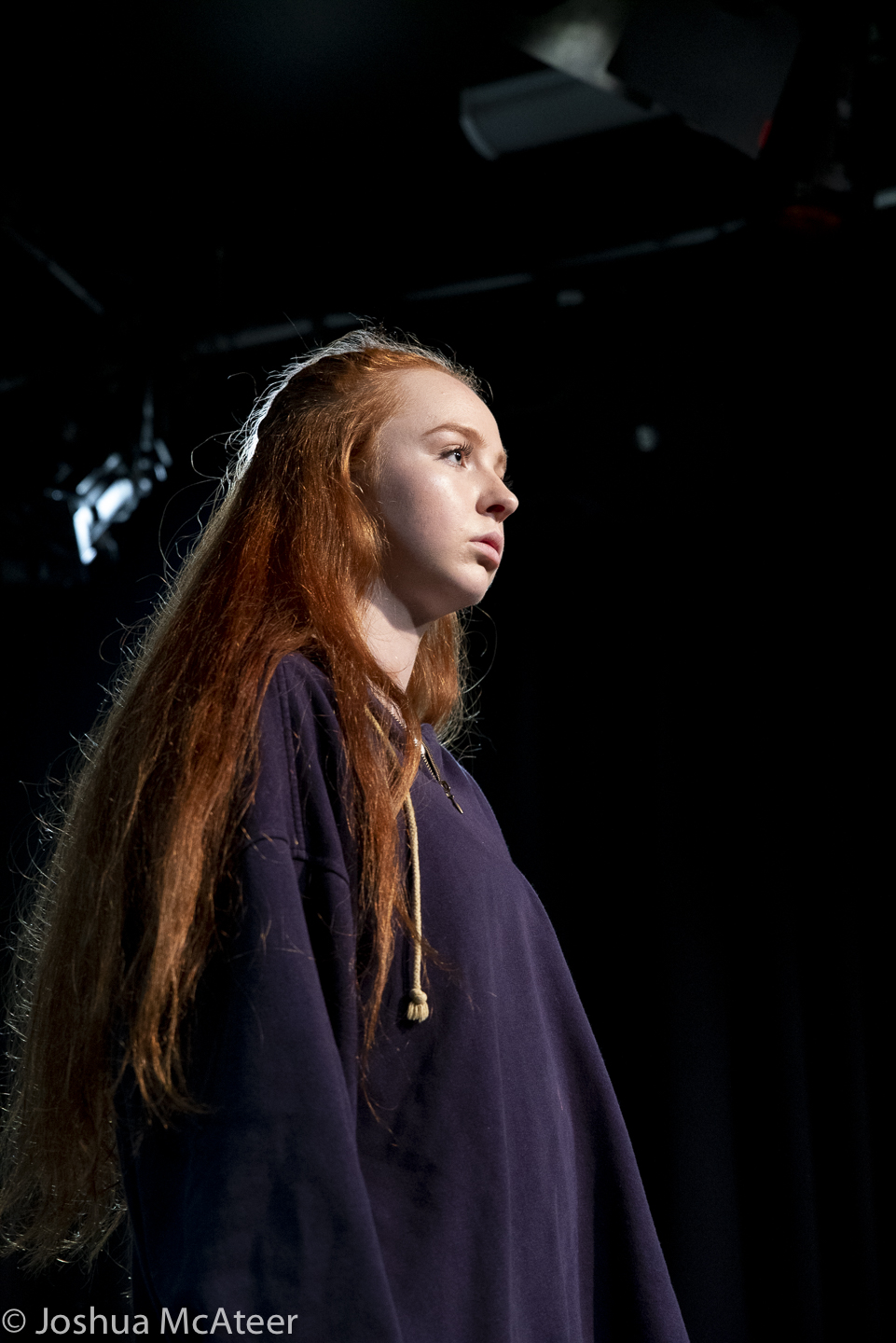
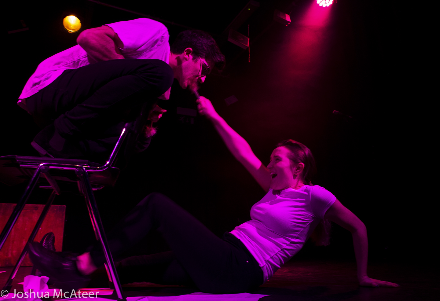
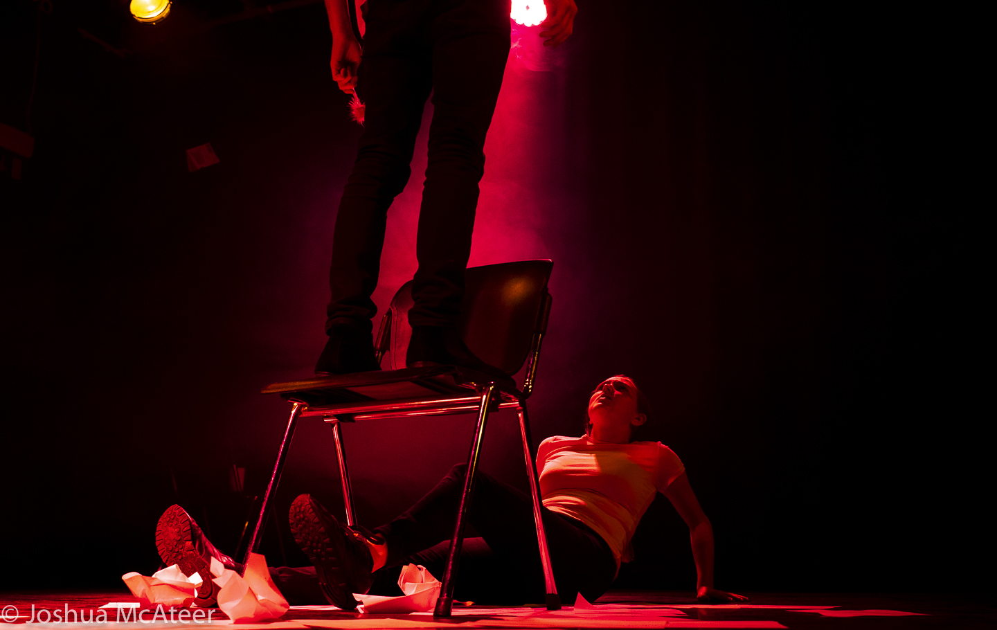
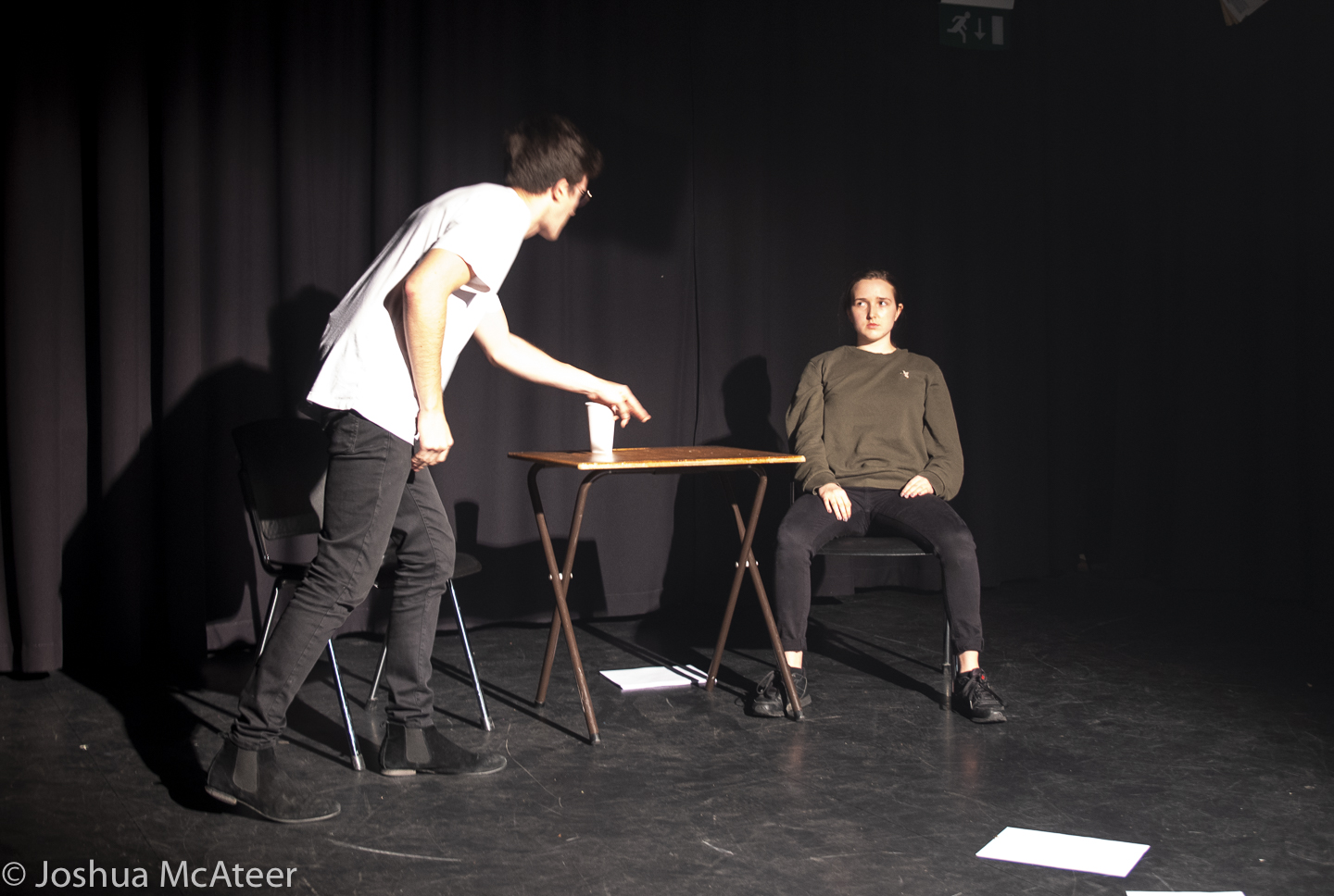
On Sunday I photographed the dress rehearsal of Heather, by the Nottingham New Theatre. The play was written by Thomas Eccleshare, and directed by Tara Phillips. The entirely student-run, theatre put together an excellent performance. From the acting to the technical effects. 

Below are some of the photos.

More of the photos can be found https://history.newtheatre.org.uk/years/18_19/heather/

Flowers on glass

Photography

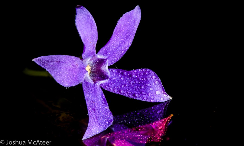
I had a specific idea in mind for this collection of photographs, an idea which I will be expanding on in the future. These are all set up single light images which have been focus stacked. I almost really like the last of these images with the daisy. However I can’t get it to look quite right. There is a reason it is called filename-Edit-edit-3.tif.

Theses shots were all taken with a studio flash head and a manual macro rail. Adjusting the focus, waiting for the vibrations to stop, taking a photo, adjusting the focus… takes a long time. I’ve since built an automated focusing rail which is much more accurate and leaves me free to make a cup of tea.

The depth of focus in macrophoto is tiny. It is even narrower when using a microscope. In microscopy ‘optical sectioning’ is a vital tool in resolving 3D structure. However, in macrophotography we often want to take front-to-back pin-sharp images. For this, we take hundreds of photos, align them, and merge them so that only the in focus details are included. Luckily, there is software for this, but if you look at the photo of the daisy up close, you’ll see how this can go badly wrong.

Skittleiser

Projects

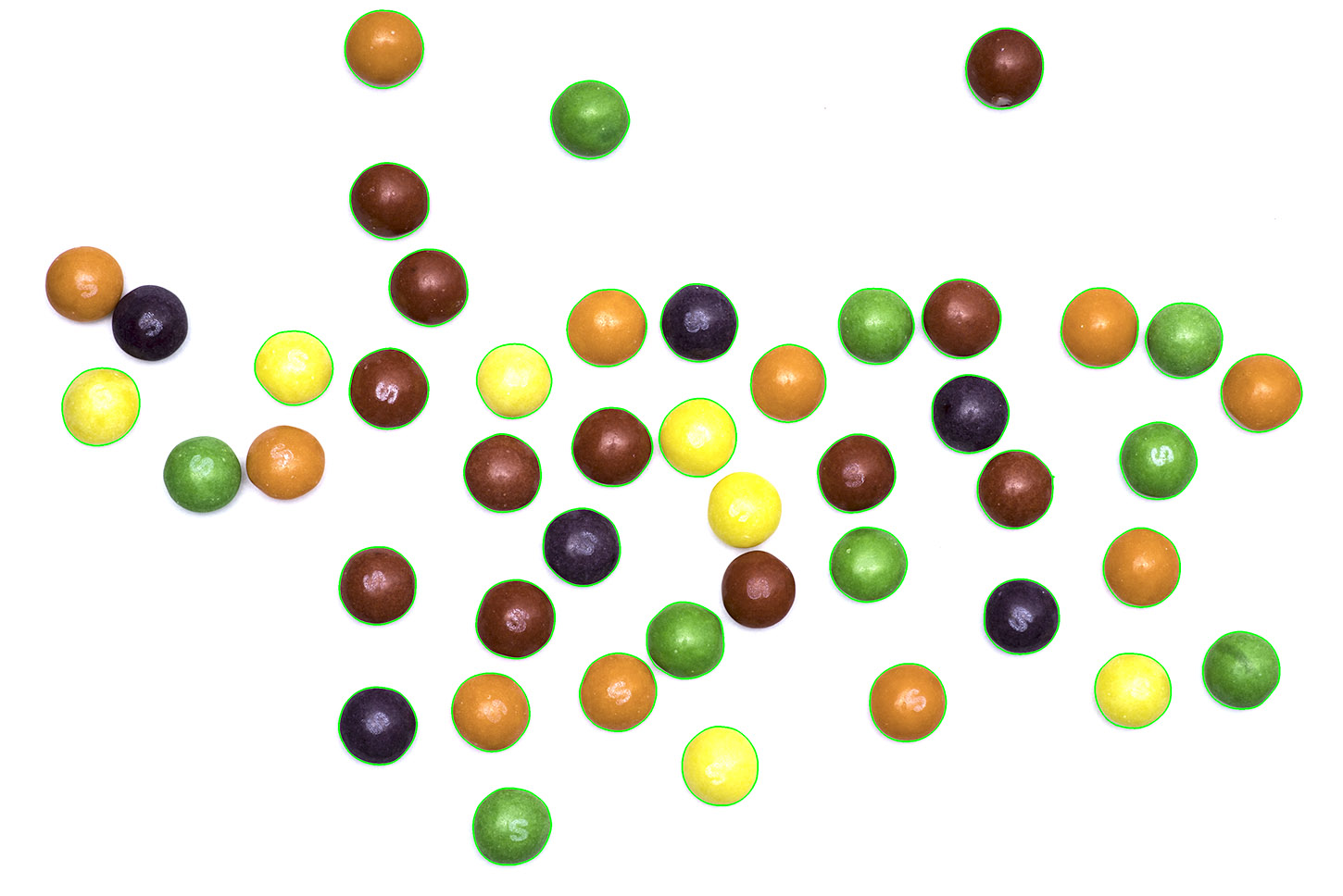
In this short project, which I finished in December of 2017, I took colour photos and represented them using images of skittles. To start off, I found photographs of skittles on the internet and segmented out the skittles manually. I was going to use my own images, but there are some flavours of skittles, which I couldn’t find at the time, and I wanted to get started right away. Since then, I have produced a library of my own skittle photos. 

There were I found eight skittle colours in total: blue, green, orange, pink, purple, white, yellow, and red. The purple skittles are very dark and look like black in contrast to the other colours. In a short python programme, I extracted small chips of an input photo and compared it to the images of the skittles. The programme then rotated the skittle image through 90, 180, and 270 degrees to see which was were best fit for the photo chip. These skittle images were then saved.

I quickly swapped to using my own skittle images, where possible. On a sheet of white paper and with a flash I took some photos of the contents of a small packet of skittles. For some reason, after each shot, the number of remaining skittles decreased. In another short python script, I used the open computer vision library to segment out the skittles and save them. I used a few steps to do this. I collapsed the images to greyscale and then blurred it and thresholded the image to produce a black and white image. This created white and black regions which corresponded to the location of the skittles, but also found regions in the background made up of noise. I then used two morphological operations, an erosion followed by a dilation. Erosion makes make black regions smaller by a set amount, and dilation makes those regions larger again. This is very useful for removing small regions in image processing tasks, like noise. Noise regions are often small enough to be removed completely when eroded, and the larger skittles are only reduced in size. I then found the location of the edges of the black regions and used this to cut out the skittles.

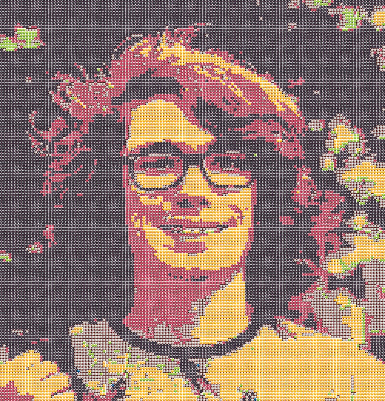
So, how delicious would portraits made out of skittles be? Well, I don’t know, as I never made any out of actual skittles. To get a decent, recognisable image you need about 10 kS (that’s kiloSkittles), or around 100 skittles on the short edge. Since skittles are about 1cm wide, it would be quite a large structure. On top of that, skittles also weigh about a gram, which would mean you’d need ~10kg of skittles, and at a penny a sweet you’d spend £100. That assumes that you can bulk buy the correct colours, which isn’t the case, most of the images I produced are mostly purple or yellow, with very little green. 

Bulk buying individual colours would make it feasible, but still not trivial. And then there’s the placing of >10 kS, although I can see that being quite therapeutic. I assumed that setting them in resin would be sufficient to preserve them, their high sugar content and a lack of oxygen should probably stop them from changing much over months, but I don’t know what might happen over a period of years.

If I ever revisit the idea I’ll add a hexagonal stacking mode, as well as the option to include dithering for greater colour accuracy. I have already added functionality for rectangular images of skittles from the side, to increase the resolution of the image in one direction. This worked, but the results weren’t as pleasing. I imagine, with the skittles on their sides, it would be that much harder to assemble. 

Dithering is an interesting concept. This medium renders images in an unusual way. If we forget about photons, the intensity of light on a given area is a continuous property, it could be twice as much as another area, or half as much, or any fraction. Digital cameras quantise this level when the analogue signal (a voltage) is converted to a digital level in a range. On dSLRs this is range is typically 12-14 bits or between 4096 and 16,384 levels. This is often then down-converted to 8 bits (256 levels) if the image is saved as a jpg, but the full range is sometimes kept with other file types. 

256 intensity levels for each colour channel is sufficient for viewing or printing images. The ability of the eye to differentiate between intensity levels is dependent on a large number of factors, including the absolute intensity of the source, as well as the colour. Colour photos allow the representation of a large number of colours and shades, typically 16.8 million. These colours can be represented in Hue, Saturation, Value or HSV space. HSV breaks down a pixel into its ‘value’, the brightness of the pixel, ‘hue’ the pure colour of the pixel, and ‘saturation’ which is how vivid the colour is, or how much of the pure colour is mixed with white. Now, our skittles well sample the different hues which are in photos, but they do not well sample any of the other dimensions of HSV space. Purple skittles are the only dark skittles, and the rest of them are all highly saturated bright colours, save for white, which is still bright. Because of this, many images cannot be well represented by skittles (I know, who’d have thought that?).

This is where dithering comes in. Dithering, in this case, trades of spatial resolution for better colour representation. A small image patch is considered, and the average colour in that patch is matched to several skittles. A light pink area, without dithering, would be represented as (say) four white skittles. But with dithering, one or two of the skittles could be swapped to red or pink. When viewed from a distance this would look much like a lighter pink. This would allow for areas of tone which are all similar to skittle colours to show some detail, and also allow for more accurate representation of the colour of image regions which are not well represented by skittle colours. 

Dithering does have some disadvantages. You lose spatial resolution, as boundaries between colours are blurred to intermediate values. It also doesn’t make ‘sense’ when viewed close up. A flat light pink region of an image may have a bright red skittle in the middle of it, and it might not be obvious from the original image why it is there.

I quite like them, anyway.

A landscape photograph overlooking a lake
A portrait of myself.
A board of the segmented skittles.